Setting Up the UHFLI Boxcar Averager for Pulsed Laser Experiments

Posted On: 14 Sep 2023

Boxcar averagers (sometimes also known with the name of “gated integrators”) are instruments used to measure signals stemming from low-duty-cycle experiments.

The information contained in low-duty-cycle pulsed signals is concentrated within a short time duration; thus, the idea behind the boxcar averager is to record the signal only during the time window where the information is present while ignoring everything outside of it – i.e. only noise.
For a comprehensive analysis of the boxcar averager and its working principles, take a look at our Principles of Boxcar Averaging white paper and related video.

The Zurich Instruments UHF-BOX Boxcar Averager (upgrade option to the UHFLI 600 MHz Lock-in Amplifier) equips the user with two independent digital boxcar averager units, configurable either with the LabOne user interface or the APIs. The purpose of this blog post is to provide practical guidance for setting up the units, optimizing your measurements, and extracting the maximum benefit from pulsed signal detection, utilizing all the advantages of digital signal processing.

Introduction

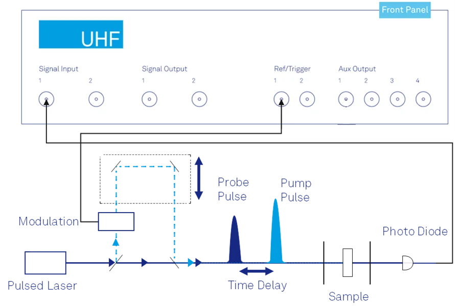
In optics and photonics applications, a widespread example of low-duty-cycle experiments is Pump-probe spectroscopy (sketch in Figure 1). This technique consists of exciting the sample with a first laser pulse, the pump, thereby promoting it to some excited state. The dynamics of this excited state can then be investigated by the interaction with a second pulse, the probe; by measuring the relative pump-induced intensity variations on the probe pulses (often denoted as ΔA/A, where A represents the intensity of the probe pulses) as a function of the time delay between the pump and the probe, one can then reconstruct the time-dependent dynamics of the excited state. One of the most important advantages of this technique lies in the fact that the time resolution is limited only by the duration of the laser pulses.

For this reason, pump-probe spectroscopy has nowadays become extensively used to study ultrafast phenomena, with many different experimental variations originating from it – e.g. Stimulated Raman Scattering (SRS) and Terahertz Time-domain spectroscopy.
However, due to the high nonlinearity of the investigated processes, the magnitude of the signals from these experiments turns out to be exceptionally small (relative variations ΔA/A down to 10^-6 or smaller). Therefore, proper signal analysis is key to achieving high signal-to-noise ratios (SNR) and ensuring proper extraction of the information from the measurements.

To maximize time resolution, many experimental instances of pump-probe spectroscopy make use of ultrashort laser pulses, running at repetition rates ranging from a few kHz to 10s of MHz and measured by fast photodetectors. Such a configuration leads to signals whose duty cycle is extremely low, e.g. 100 fs pulses running at 100 kHz repetition rate detected with a 100 MHz photodetector (i.e. 10 ns rise time) result in a duty cycle of about 0.1% – the duty cycle being defined as PW*100/T, where PW is the pulse width and T is the inverse of the repetition rate.
Consequently, in these cases, boxcar averaging becomes the better measurement approach leading to the best signal-to-noise ratio.

Figure 1: Typical experimental layout of pump-probe spectroscopy.

The procedure to configure the UHF-BOX Boxcar averager in a more general case is thoroughly explained in this video.

Here, we focus on the specific case of pulsed laser spectroscopy, with emphasis on two common use cases, covering most of the experimental configurations.
A key experimental parameter is the frequency at which the pump beam is modulated, in turn defining the frequency at which our signal appears on top of the probe pulses.
Whenever feasible, it is always advisable to choose the modulation frequency as high as possible, the upper limit being half the repetition rate of the laser itself (i.e., one pulse “ON” and one pulse “OFF”). In fact, this condition minimizes the impact of correlated and 1/f noise contributions and only noise which is uncorrelated from one laser shot to the next remains. However, depending on the specific experimental configuration, high modulation frequencies might not be always achievable.

Therefore, the possible scenarios are:

1. The modulation frequency of the pump beam is exactly ½ the repetition rate of the laser, f_mod = f_rep/2.
2. The modulation frequency of the pump beam is < ½ the repetition rate of the laser, f_mod < f_rep/2

Case 1

Next to the best noise performance, this scenario has also the great advantage of allowing the user to set up the Boxcar units to directly obtain the relative intensity variations normalized by the intensity of the probe pulses (i.e., ΔA/A) as the output of the measurement.

Let’s suppose now to connect the voltage output of our photodiode to the Signal Input 1 of the UHFLI and visualize it on the Oscilloscope. Additionally, we provide the reference frequency, f_mod, from the modulator — e.g., the “Sync” signal from the chopper or the driving signal to the Acousto-optic modulator (AOM) or Electro-optic modulator (EOM), in the example below about 72 kHz — to one of the Ref/Trigger Inputs. The instrument then phase-locks to it by activating the ExtRef mode of Demodulators 4 or 8.
It is worth mentioning that the driving signal to the modulator can also be provided by the UHFLI itself, via one of the two Signal Outputs or as a TLL signal from one of the Trigger Outputs.

Figure 2: Lock-in tab with external reference connected to Trigger 1 and locked to Oscillator 4.

When f_mod = f_rep/2, every second pulse carries the information of the interaction with the sample. This can be seen in the exemplary scope shot of Figure 3, where every subsequent pulse has a smaller amplitude – the effect is exaggerated for visualization purposes; as mentioned before, these amplitude variations are normally on the order of parts per million or smaller.

Figure 3: Scope shot of a simulated pulsed signal from a photodiode.

If we now analyze the signal with the embedded Periodic Waveform Analyzer (PWA) of the Boxcar units, we can plot a single period of the reference frequency f_mod, whereby two subsequent pulses will come into view. We can then configure both Boxcar units to lock to the same oscillator (the one locked to f_mod) and use unit 1 to measure the difference between these two pulses, i.e. ΔA, by enabling the Baseline Subtraction option, and unit 2 to record only the magnitude of the pulses for normalization, i.e. A. Even though in Boxcar unit 2 we are now only interested in measuring one of the pulses in the period, it is nevertheless advisable to enable the baseline subtraction option, placing the window somewhere in the period where no signal is present, to eliminate any potential DC or slowly varying component. Figure 4 shows the configuration of the two units, respectively.

Figure 4: Configuration of Boxcar units 1 and 2. Unit 1 carries the information about ΔA and unit 2 about A.
The signal in the PWA can be plotted as a function of phase or time.

It is worth noting that, in a real experiment where the difference between the two pulses is extremely small, the order of the subtraction and the pulse chosen for normalization don’t play a significant role.

One can then perform the normalization with the Arithmetic Unit of the UHFLI, by setting one of the cartesian units to perform the ratio between Boxcar 1 and Boxcar 2 results, as shown in Figure 5, left panel.
Importantly, to make sure that the normalization is consistent, it should be performed pulse by pulse. This means that the averaging period on both Boxcar units should be set to 1 (i.e., no averaging of subsequent pulses should be performed), as shown in Figure 4 highlighted in orange.

Figure 5: Arithmetic Unit (left panel) and Auxiliary Output configuration (right panel).

At this point, the output of the Arithmetic Unit is the result of the measurement (ΔA/A) and it can either be saved on the host computer – making sure to have set the Arithmetic Unit Data Transfer rate that is at least twice as much as the corresponding averaging bandwidth — or output out of the instrument via the Auxiliary Outputs of the UHFLI, with custom scaling and offset. To increase the signal-to-noise ratio, the measurement result ΔA/A can then be averaged over many periods by post-processing. Simultaneously, it is also possible to output the results of the individual Boxcar units (see Figure 5, right panel) and/or visualize the measurement as a function of time with the Plotter tool as displayed in Figure 6.

Figure 6: Visualization of the Arithmetic Unit measurement result, proportional to ΔA/A.

Case 2

If f_mod < f_rep/2, the signal from the photodiode carries a signal component at the modulation frequency, f_mod, on top of the laser pulses at f_rep. In Figure 7, a shot from the oscilloscope shows an example of such a scenario, where the repetition rate of the laser is about 10 times larger than the modulation frequency.

Figure 7: Signal plotted on the oscilloscope, where f_mod and f_rep can be identified. The effect of the modulation is exaggerated for the sake of visualization.

In this case, a 2-step approach is necessary:

1. Lock one of the Boxcar units to the repetition rate of the laser f_rep and measure the intensity of all the pulses arriving at the detector
2. Perform a lock-in measurement on the result of the boxcar measurement above, demodulating it at the modulation frequency, f_mod

To this end, we need to provide both f_mod and f_rep to the instrument. As shown in Figure 7, these two external references can be connected to e.g., Trigger 1 and Trigger 2 respectively.

Figure 8: PWA running at the f_rep, resulting in a single pulse within the period. The averaging bandwidth must be larger than f_mod to ensure proper reconstruction of the modulated signal.

In this situation, it is essential to ensure that the resulting averaging bandwidth of the boxcar measurement, adjustable with the number of averaging periods, is larger than f_mod — in the example above, f_mod is 10 kHz and the averaging bandwidth is set to 50 kHz. In fact, if this weren’t the case, the signal component at f_mod would be suppressed. The setup of the Boxcar averager parameters for this case is shown in Figure 8.

If we now use the Plotter tool to visualize the output of the Boxcar unit as a function of time, we can clearly observe the signal being periodic, with a period equal to 1/f_mod (see Figure 9). Here, to guarantee proper reconstruction of the signal in the Plotter the Rate limit in Samples/s (and in turn the Rate) should be high enough to properly resolve the frequency of the signal. This translates in the condition where Data Transfer Rate (Sa/s) > 2*f_mod.

Figure 9: Result of the boxcar measurement, with a clear periodic signal at a frequency f = f_mod

At this point, we can internally redirect the output of Boxcar unit 1 to one of the Aux Outputs and in turn use this signal as the input of one of the demodulators in the lock-in tab, with the demodulation frequency set at f_mod. This procedure is highlighted in Figure 10.
The result of this demodulation is then directly proportional to ΔA.

Note that the signal rerouting happens internally hence the best SNR is extracted with high numerical precision in a minimal amount of time. Additionally, it is also worth mentioning that this rerouting is not affected by the Rate or Rate limit parameters of the Boxcar units, as the Aux Output is always sampled at 28 MSa/s, regardless of whether the signal is then internally rerouted or physically output from the instrument.

Figure 10: Rerouting of the signal to one of the Aux Out (top) and subsequent demodulation with one of the demodulators, running at f_mod. In the bottom panel, the result of such demodulation visualized with the Plotter tool.

Unlike case 1, when f_mod < f_rep/2, the signal normalization by the pulses’ amplitude turns out to be not straightforward. Retrieving a properly normalized ΔA/A requires the measurement of the pulses’ intensity without the pump-induced contribution, i.e. A, in an equivalent way as measured for ΔA. This procedure might require sizable changes to the optical setup to ensure consistency and uniformity between the measurement of ΔA and A.

Conclusion

In conclusion, we have seen how to configure the UHF-BOX Boxcar averagers units, and more generally the UHFLI, depending on the modulation frequency of the experiment, f_mod. If such frequency is = ff_rep/2, then a fully differential measurement with baseline subtraction and pulse intensity normalization is possible, with the measurement output representing the relative pump-induced intensity variations on the probe pulses, i.e. ΔA/A.

In any other case, when f_mod < f_rep/2, a two-step approach is necessary, first integrating the pulses with one of the Boxcar units and then demodulating its output with one of the instruments’ digital demodulators, ending up with a signal proportional to ΔA.